How big is the “average” protein?

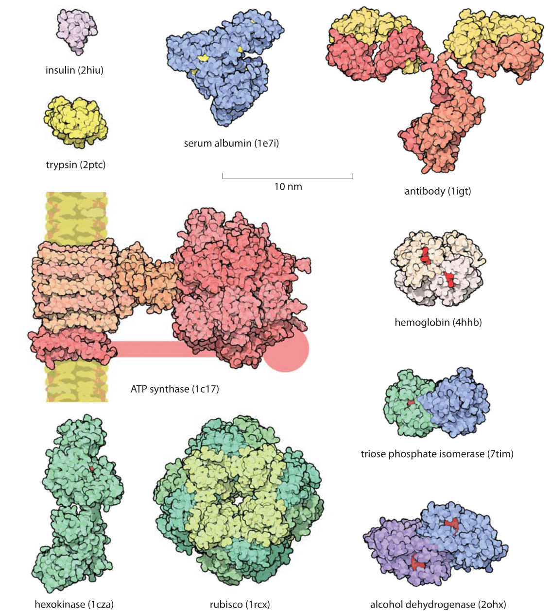
Figure 1: Gallery of proteins. Representative examples of protein size are shown with examples drawn to illustrate some of the key functional roles they take on. All the proteins in the figure are shown on the same scale to give an impression of their relative sizes. The small red objects shown on some of the molecules are the substrates for the protein of interest. For example, in hexokinase, the substrate is glucose. The handle in ATP synthase is known to exist but the exact structure was not available and thus only schematically drawn. Names in parenthesis are the PDB database structures entries IDs. (Figure courtesy of David Goodsell).

Proteins are often referred to as the workhorses of the cell. An impression of the relative sizes of these different molecular machines can be garnered from the gallery shown in Figure 1. One favorite example is provided by the Rubisco protein shown in the figure that is responsible for atmospheric carbon fixation, literally building the biosphere out of thin air. This molecule, one of the most abundant proteins on Earth, is responsible for extracting about a hundred Gigatons of carbon from the atmosphere each year. This is ≈10 times more than all the carbon dioxide emissions made by humanity from car tailpipes, jet engines, power plants and all of our other fossil-fuel-driven technologies. Yet carbon levels keep on rising globally at alarming rates because this fixed carbon is subsequently reemitted in processes such as respiration, etc. This chemical fixation is carried out by these Rubisco molecules with a monomeric mass of 55 kDa fixating CO₂ one at a time, with each CO₂ with a mass of 0.044 kDa (just another way of writing 44 Da that clarifies the 1000:1 ratio in mass). For another dominant player in our biosphere consider the ATP synthase (MW≈500-600 kDa, BNID 106276), also shown in Figure 1, that decorates our mitochondrial membranes and is responsible for synthesizing the ATP molecules (MW=507 Da) that power much of the chemistry of the cell.  These molecular factories churn out so many ATP molecules that all the ATPs produced by the mitochondria in a human body in one day would have nearly as much mass as the body itself. As we discuss in the vignette on “What is the turnover time of metabolites?” the rapid turnover makes this less improbable than it may sound.

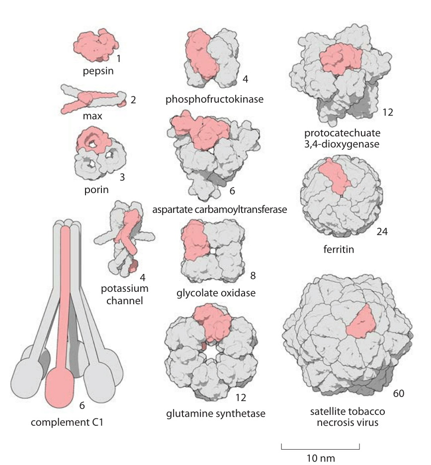
Figure 2: A Gallery of homooligomers showing the beautiful symmetry of these common protein complexes. Highlighted in pink are the monomeric subunits making up each oligomer. Figure by David Goodsell.

The size of proteins such as Rubisco and ATP synthase and many others can be measured both geometrically in terms of how much space they take up and in terms of their sequence size as determined by the number of amino acids that are strung together to make the protein. Given that the average amino acid has a molecular mass of 100 Da, we can easily interconvert between mass and sequence length. For example the 55 kDa Rubisco monomer, has roughly 500 amino acids making up its polypeptide chain. The spatial extent of soluble proteins and their sequence size often exhibit an approximate scaling property where the volume scales linearly with sequence size and thus the radii or diameters tend to scale as the sequence size to the 1/3 power. A simple rule of thumb for thinking about typical soluble proteins like the Rubisco monomer is that they are 3-6 nm in diameter as illustrated in Figure 1 which shows not only Rubisco, but many other important proteins that make cells work. In roughly half the cases it turns out that proteins function when several identical copies are symmetrically bound to each other as shown in Figure 2. These are called homo-oligomers to differentiate them from the cases where different protein subunits are bound together forming the so-called hetero-oligomers. The most common states are the dimer and tetramer (and the non oligomeric monomers). Homo-oligomers are about twice as common as hetero-oligomers (BNID 109185).

There is an often-surprising size difference between an enzyme and the substrates it works on. For example, in metabolic pathways, the substrates are metabolites which usually have a mass of less than 500 Da while the corresponding enzymes are usually about 100 times heavier. In the glycolysis pathway, small sugar molecules are processed to extract both energy and building blocks for further biosynthesis. This pathway is characterized by a host of protein machines, all of which are much larger than their sugar substrates, with examples shown in the bottom right corner of Figure 1 where we see the relative size of the substrates denoted in red when interacting with their enzymes.

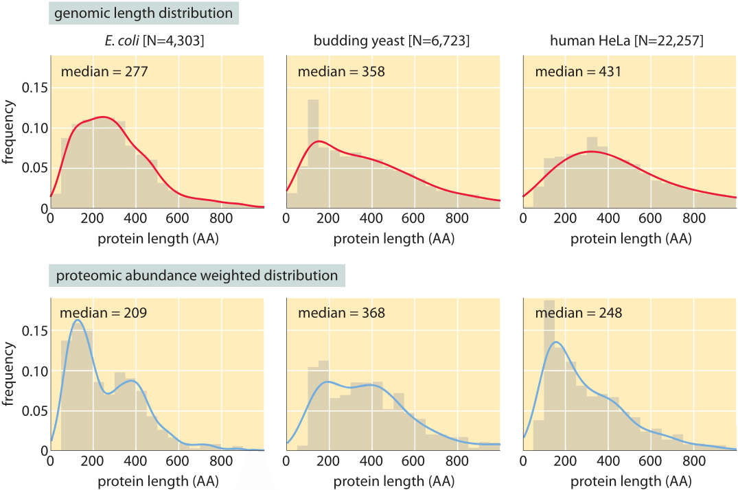
Figure 3: Distribution of protein lengths in E. coli, budding yeast and human HeLa cells. (A) Protein length is calculated in amino acids (AA), based on the coding sequences in the genome. (B) Distributions are drawn after weighting each gene with the protein copy number inferred from mass spectrometry proteomic studies (M. Heinemann in press, M9+glucose; LMF de Godoy et al. Nature 455:1251, 2008, defined media; T. Geiger et al., Mol. Cell Proteomics 11:M111.014050, 2012). Continuous lines are Gaussian kernel-density estimates for the distributions serving as a guide to the eye.

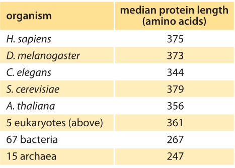
Table 1: Median length of coding sequences of proteins based on genomes of different species. The entries in this table are based upon a bioinformatic analysis by L. Brocchieri and S. Karlin, Nuc. Acids. Res., 33:3390, 2005, BNID 106444. As discussed in the text, we propose an alternative metric that weights proteins by their abundance as revealed in recent mass spec proteome-wide censuses. The results are not very different from the entries in this table, with eukaryotes being around 400 aa long on average and bacteria about 300 aa long.

Concrete values for the median gene length can be calculated from genome sequences as a bioinformatic exercise. Table 1 reports these values for various organisms showing a trend towards longer protein coding sequences when moving from unicellular to multicellular organisms. In Figure 3 we go beyond mean protein sizes to characterize the full distribution of coding sequence lengths on the genome, reporting values for three model organisms. If our goal was to learn about the spectrum of protein sizes, this definition based on the genomic length might be enough. But when we want to understand the investment in cellular resources that goes into protein synthesis, or to predict the average length of a protein randomly chosen from the cell, we advocate an alternative definition, which has become possible thanks to recent proteome-wide censuses. For these kinds of questions the most abundant proteins should be given a higher statistical weight in calculating the expected protein length. We thus calculate the weighted distribution of protein lengths shown in Figure 3, giving each protein a weight proportional to its copy number. This distribution represents the expected length of a protein randomly fished out of the cell rather than randomly fished out of the genome. The distributions that emerge from this proteome-centered approach depend on the specific growth conditions of the cell. In this book, we chose to use as a simple rule of thumb for the length of the “typical” protein in prokaryotes ≈300 aa and in eukaryotes ≈400 aa. The distributions in Figure 3 show this is a reasonable estimate though it might be an overestimate in some cases.

One of the charms of biology is that evolution necessitates very diverse functional elements creating outliers in almost any property (which is also the reason we discussed medians and not averages above). When it comes to protein size, titin is a whopper of an exception. Titin is a multi-functional protein that behaves as a nonlinear spring in human muscles with its many domains unfolding and refolding in the presence of forces and giving muscles their elasticity. Titin is about 100 times longer than the average protein with its 33,423 aa polypeptide chain (BNID 101653).  Identifying the smallest proteins in the genome is still controversial, but short ribosomal proteins of about 100 aa are common.

It is very common to use GFP tagging of proteins in order to study everything from their localization to their interactions. Armed with the knowledge of the characteristic size of a protein, we are now prepared to revisit the seemingly innocuous act of labeling a protein. GFP is 238 aa long, composed of a beta barrel within which key amino acids form the fluorescent chromophore as discussed in the vignette on “What is the maturation time for fluorescent proteins?”. As a result, for many proteins the act of labeling should really be thought of as the creation of a protein complex that is now twice as large as the original unperturbed protein.