How fast are electrical signals propagated in cells?
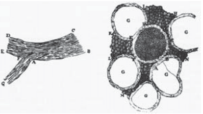
Figure 1: Antoine van Leeuwenhoek’s 1719 drawings of nerve cells in a letter to a friend. The drawing on the left shows a longitudinal view of nerves and the drawing on the right shows a cross-sectional view of a central nerve surrounded by five others (labeled with “G”). (Adapted from: F. Lopez-Munoz et al., Brain Res. Bul. 70:391, 2006.)
Nerve cells are among the most recognizable of human cell types, noted not only for their enormous size relative to many of their cellular counterparts, but also for their unique shapes as revealed by their sinuous and elongated structures. Already in the early days of microscopy, biological pioneers found these cells a fascinating object of study, with van Leeuwenhoek musing, “Often and not without pleasure, I have observed the structure of the nerves to be composed of very slender vessels of an indescribable fineness, running length-wise to form the nerve”. See Figure 1 for several examples of the drawings made by van Leeuwenhoek as a result of his observations with the early microscope. The mystery of nerve cells went beyond their intriguing morphology as a result of their connection with electrical conduction and muscle action. In famed experiments like those shown in Figure 2, Luigi Galvani discovered that muscles in dead frogs could be stimulated to twitch by the application of an electrical shock. This work set the stage for several centuries of work on animal electricity culminating in our modern notions of the cellular membrane potential and propagating action potentials. These ideas now serve as the cellular foundation of modern neuroscience.
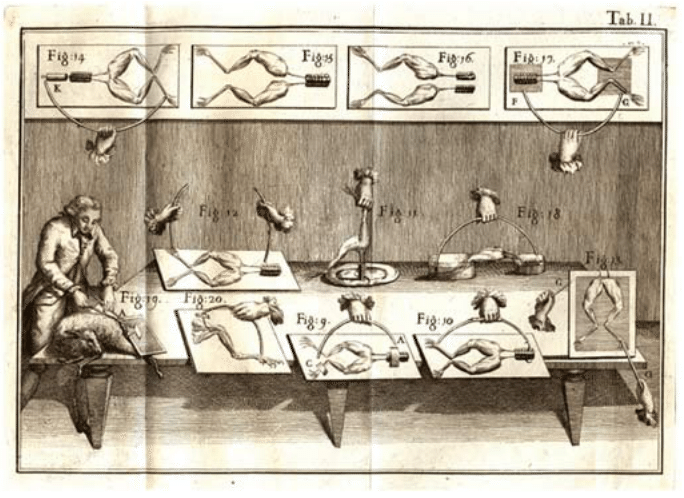
Figure 2: The experiments of Luigi Galvani on the electrical stimulation of muscle twitching. Using a dead frog, Galvani discovered that he could use an electrical current to induce muscle twitching, lending credence to the idea that nervous impulses are electrical. Figure adapted from Galvani’s book De Viribus Electricitatis in Motu Musculari (1792).
![Figure 3: The measurements of Herman von Helmholtz on the propagation of nervous impulses. Schematic of the apparatus used by Helmholtz in his measurments. The stimulated nerve was used to lift the wegiht shown at the bottom of the apparatus. (Adapted from Helmholtz H [1850] Archiv fur Anatomie, physiologie und wissenschaftliche Medicin MPIWG:2AT3G7QD. courtesy of the Max Planck Institute for History of Science.)](http://book.bionumbers.org/wp-content/uploads/2014/08/CBBTN_Ch4-38-page-0.jpg)
Figure 3: The measurements of Herman von Helmholtz on the propagation of nervous impulses. Schematic of the apparatus used by Helmholtz in his measurments. The stimulated nerve was used to lift the wegiht shown at the bottom of the apparatus. (Adapted from Helmholtz H [1850] Archiv fur Anatomie, physiologie und wissenschaftliche Medicin MPIWG:2AT3G7QD. courtesy of the Max Planck Institute for History of Science.)
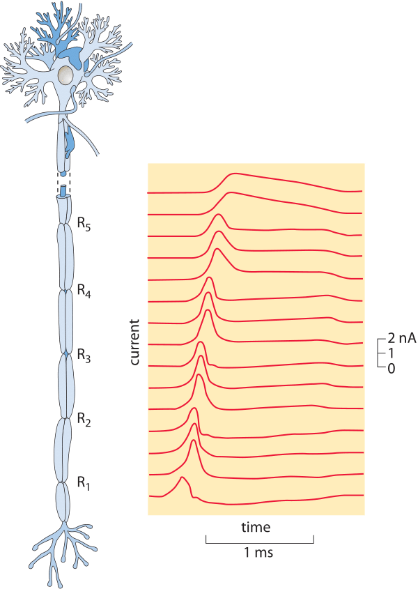
Figure 4: Measurement of the propagation of a nervous impulse. (Adapted from A. F. Huxley and R. Stampfli, J. Physiol. 108:315, 1949.)
In the time since, numerous measurements have confirmed and extended the early insights of Helmholtz with a broad range of propagation speeds ranging from less than a meter per second all the way to over a hundred of meters per second (the fastest taking place in a shrimp giant fiber with a value over half of the speed of sound! (BNID 110502, 110597). Figure 4 shows the results of one of these classic studies. Determining the mechanistic underpinnings of variability in the speed of nervous impulses has been one of the preoccupations of modern neurophysiology and has resulted in insights into how both the size and anatomy of a given neuron dictate the action potential propagation speed. An important insight that attended more detailed investigations of the conduction of nervous impulses was the realization that the propagation speed depends both on the cellular anatomy of the neuron in question such as whether it has a myelin sheath (increasing the propagation speed several fold) and also on the thickness of the nerve (propagation speed being proportional to the diameter in myelinated neurons and proportional to the area in unmyelinated neurons).
Early work on impulse conduction along peripheral fibers by Erlanger and Gasser, for which they shared the Nobel Prize in 1942, demonstrated remarkable relationships between the conduction velocity of the axons and the type of neuron and thus the information that they conveyed. The largest motor fibers (13-20 μm, conducting at velocities of 80-120 m/s) innervate the extrafusal fibers of the skeletal muscles, and smaller motor fibers (5-8 μm, conducting at 4-24 m/s) innervate intrafusal muscle fibers. The largest sensory fibers (13-20 μm) innervate muscle spindles and Golgi tendon organs, both conveying unconscious proprioceptive information. The next largest sensory fibers (6-12 μm) convey information from mechanoreceptors in the skin, and the smallest myelinated fibers (1 –5 μm) convey information from free nerve endings in the skin, as well as pain, and cold receptors.
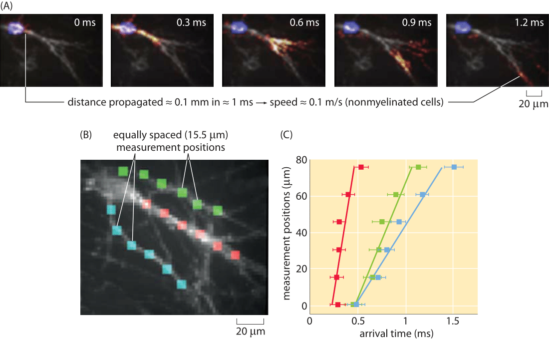
Figure 5: Optical measurement of action potential speed. (A) Series of images of the fluorescence in the cell as a function of time. (B) A series of equally spaced (15 μm) measurement points along three different processes are used to measure the arrival time of a propagating action potential. (C) Arrival times for the three processes shown in part (B). For example, for the action potential propagating along the fiber labeled with red boxes, the signal arrives with a time delay of roughly 0.05 ms from one measurement point to the next. The action potential speed can be read off of the graph in the usual wayby dividing distance traveled by time elapsed. Note that due to technical limitations these are unmyelinated neuronal cells and thus the propagation speed is much slower than in-vivo. (Figure courtesy of Daniel Hochbaum and Adam Cohen.)
One of the beautiful outcomes of recent fluorescent methods is the invention of genetically encoded voltage reporters. These molecular probes have differing fluorescence depending upon the membrane voltage. An impressive usage of these methods has been to watch in real time the propagation of nerve impulses. Specifically, the readout of the passing of such an impulse comes from the transient change in fluorescence along the neuron. An example of this method is shown in Figure 5. We note these alternative methods because of the strict importance we attach to the ability to measure the same quantity in multiple ways, especially to make sure that they yield consistent values.
Can we connect the reported action potential speeds in humans of 10-100 m/s (BNID 110594) to our human response limits? From the moment of hearing the firing of the starter’s pistol in a 100-meter dash to activating the muscles in the feet, at least one meter of impulse propagation had to take place. This dictates a latency of 10-100 ms even before taking into account all other latencies such as the processing happening in the brain and the propagation time due to the finite speed of sound in air. Indeed in a 100-m dash race, the best athletes have response times of roughly 120 ms (BNID 111450) and anything below 100 ms is actually disqualified as a false-start according to the binding rules of the International Association of Athletics Federations. If the propagation speed of nerve impulses were significantly slower, running races as well as soccer games or indeed most sports events would be much less interesting to watch. Speaking of watching, we know that when shown frames at the standard rate of 24 Hz the brain sees or interprets the movement as continuous. It is interesting to speculate what the frame rate would have to be if our action potentials were moving at, say, 1000 m/s.