How many chromosomes are found in different organisms?
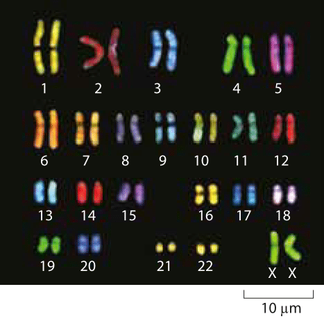
Figure 1: Microscopy images of human chromosomes. Spectral karotyping allows for the visualization of chromosomes by effectively painting each chromosome fluorescently with a different color. (Adapted from http://www.genome.gov/10000208).
The flu is one of the unfortunate realities of human health. This unpleasant (and sometimes deadly) malady results from infection by the influenza virus, a beautiful virus whose structure was already shown in the vignette on “How big are viruses?”. One of the fascinating features of these viruses is that the roughly 14,000 bases (BNID 106760) of their negative sense RNA genomes are split over 8 distinct RNA molecules (BNID 110377) demonstrating that even in the case of viruses, genomes are sometimes split up into distinct molecules. This kind of weirdness is even more strikingly demonstrated in the case of the Cowpea Chlorotic Mottle virus (CCMV) whose ≈8000 base genome is separated into three distinct RNA molecules (BNID 106457) each packed into a different capsid meaning that all three of them need to infect the host in order for the infection to be viable.
Though our favorite bacterium E. coli has only a single circular chromosome, many prokaryotes have multiple circular chromosomes. For example, Vibrio cholerae, the pathogen that is responsible for cholera has two circular chromosomes, one with a length of 2.9 Mb and the other with a length of 1.1 Mb. A more bizarre example is found in the bacterium Borrellia burgdorferi that sometimes causes Lyme disease after animals suffer a bite from a tick. This bacterium contains 11 plasmids containing 430 genes, beyond its long linear chromosome (BNID 111258). The microscopic world of Archaea seems to have similar chromosomal distributions to those found in bacteria, though M. jannaschii has three different circular DNA molecules with lengths of roughly 1.6 Mbp, 58.5 kbp and 16.5 kbp, showing again the wide and varied personalities of microbial chromosomes. The picture of microbial genomes is further complicated by the fact that our tidy picture of circular Mb-sized chromosomes is woefully incomplete since it ignores the genes that are shuttled around on small (i.e. roughly 5 kbp) plasmids.
Ultimately, for most of us, our mental picture of chromosomes is largely based upon images from eukaryotic organisms like those shown in Figure 1. As listed in Table 1 in the vignette on “How big are genomes?”, there is a great variety in the number of pairs of chromosomes in different organisms. One would think that at least the two model fungi, budding yeast and fission yeast, would show similar numbers of chromosomes. Yet surprisingly, the budding yeast S. cerevisiae has 16 chromosomes and the fission yeast S. pombe has only 3 chromosomes. Similarly, other classic model organisms do not show any consistent pattern: C. elegans (6 chromosomes), fruit fly Drosophila melanogaster (4 chromosomes) mouse Mus musculus (20 chromosomes). The comparison of budding yeast and the fly shows how a ≈10-fold larger genome in the case of Drosophila can be accommodated with ¼ as many chromosomes as the 16 found in budding yeast. Among animals the red vizcacha rat has the largest number of chromosomes at 102 (BNID 110010). These examples demonstrate that the number of chromosomes is not at all dictated by the physical size of the animal and also overturn the long-held belief that animals cannot be polyploid, as the red vizcacha rat is tetrapolid, i.e. has 4 copies of each chromosome rather than the 2 found in humans and other diploids.
As most of us learn in high school, humans have 23 pairs of chromosomes. Given the 3 x 10⁹ base pairs in the human haploid genome, this means that each chromosome harbors on average roughly 130 Mb of DNA, with the smallest, chromosome 21, carrying ≈50 Mb and the largest, chromosome 1, at ≈250 Mb. Some of the most insidious genetic diseases are the result of extra copies of these chromosomes. For example, Down’s syndrome results from an extra copy of chromosome 21 and there are more of these so-called “trisomies” associated with other chromosomes and leading to other (mainly lethal) syndromes.
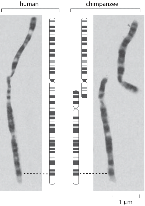
Figure 2: Chromosomal banding patterns in late-prophase chromsomes. (Adapted from J. J. Yunis and O. Prakash, Science, 215:1525, 1982.
One of the stories that elicit the most fascination in all of biology centers on the question of human evolution and its relation to chromosome number and is highlighted in Figure 2. We humans have 23 pairs of chromosomes and interestingly, chimps, gorillas and orangutans have 24 such pairs. The figure shows a comparison of the structure of chromosome 2 in humans and of two related chromosomes (called 2p and 2q) in our closest primate relative, the chimpanzee. A comparison of the banding patterns in late prophase chromosomes has been invoked as a key piece of evidence for common chromosomal ancestry (the reader is invited to examine the highly stereotyped chromosomal patterns in the rest of the chromosomes in the original papers). A head to head fusion of the 2p and 2q primate chromosomes, led to the formation of the human chromosome 2. This picture was lent much more credence as a result of recent DNA sequencing that found evidence within human chromosome 2 such as a defunct centromeric sequence corresponding to the centromere from one of the chimp chromosomes as well as a vestigial telomere on our chromosome 2. This story has garnered great interest on the internet where nonscientists that take issue with both the fact and theory of evolution espouse various refutations and untestable conspiratorial speculations on this fascinating chromosomal history.
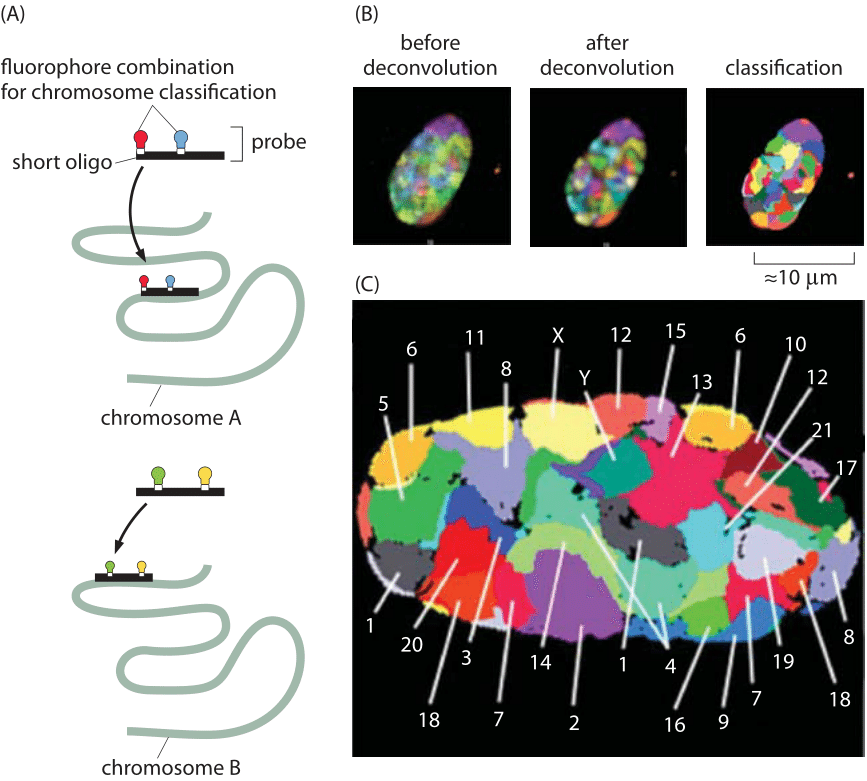
Figure 3: Localization of chromosome territories revealed using confocal microscopy. Classification of chromosomes in a Human fibroblast nucleus is based on 24-color 3D FISH experiments, Chromosome probes for all 24 chromosome types (1–22, plus X and Y) were labeled using a combinatorial labeling scheme with seven differentially labeled nucleotides. (Adapted from A. Bolzer et al. PLoS Biol., 3: e157, 2005).
Another exciting recent experimental development in the study of genome organization has been the ability to explore the relative spatial organization of different chromosomes. The existence of well-defined chromosome territories has been discovered in both prokaryotes and eukaryotes. Figure 3 shows an example for the nucleus of a human fibroblast cell. Hybridization of fluorescent probes led to the false color representation of chromosome territories in the mid-section of the nucleus. Using more recent tools known as “chromosome capture”, even the chromosome territories of the human genome have been mapped out. In these chromosome capture methods, physical crosslinking of parts of the genome that are near each other are used to build a proximity map. The maps make the chromosomes look like crumpled globules, which would not be the case if they behaved like equilibrated linear polymers but are rather the result of active structuring taking place inside the nucleus leading to nuclear and chromosomal territories. Interestingly, disorders in such territories are now suggested to cause diseases such as the very early aging in progeria due to a mutation in a critical component of the nuclear lamina that leads to displacement of some inactive genes and therefore to their upregulation (P. W. Tai et al., J Cell Physiol. 229:711, 2014). In yeast there is no proof of such structure and the use of polymer physics ideas on equilibrium polymers appears to be a valid representation. At finer resolution, chromosomes are further subdivided into “domains”. That is, parts of one chromosome are to a large extent territorially segregated from each other. This might enable the actual number of chromosomes to change quite a lot without severely affecting genome spatial regulation. Finally there is heterogeneity in location, where while chromosomes are segregated, the specific “geography” of territories might be different for either different cells, or even for one cell over time.
Despite the many interesting stories that color this vignette, we are curious to see if new research will associate any deeper functional significance to the chromosome count.