How many genes are in a genome?
We have already examined the great diversity in genome sizes across the living world (see Table in the vignette on “How big are genomes?”). As a first step in refining our understanding of the information content of these genomes, we need a sense of the number of genes that they harbor. When we refer to genes we will be thinking of protein-coding genes excluding the ever-expanding collection of RNA coding regions in genomes.
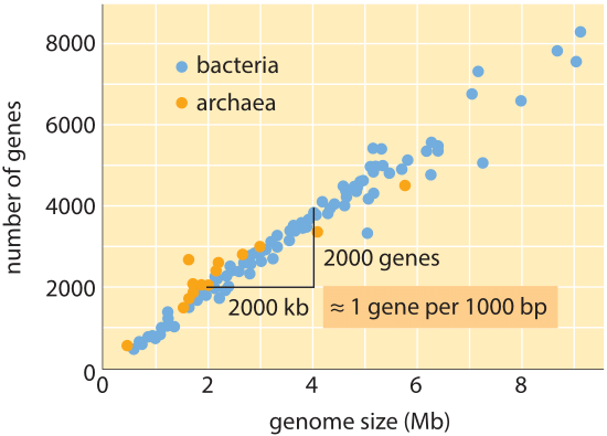
Figure 1: Number of genes as a function of genome size. The figure shows data for a variety of bacteria and archaea, with the slope of the data line confirming the simple rule of thumb relating genome size and gene number. (Adapted from M. Lynch, The Origins of Genome Architecture.)
Over the whole tree of life, though genome sizes differ by as much as 8 orders of magnitude (from <2 kb for Hepatitis D virus (BNID 105570) to >100 Gbp for the Marbled lungfish (BNID 100597) and certain Fritillaria flowers (BNID 102726)), the range in the number of genes varies by less than 5 orders of magnitude (from viruses like MS2 and QB bacteriophages having only 4 genes to about one hundred thousand in wheat). Many bacteria have several thousand genes. This gene content is proportional to the genome size and protein size as shown below. Interestingly, eukaryotic genomes, which are often a thousand times or more larger than those in prokaryotes, contain only an order of magnitude more genes than their prokaryotic counterparts. The inability to successfully estimate the number of genes in eukaryotes based on knowledge of the gene content of prokaryotes was one of the unexpected twists of modern biology.
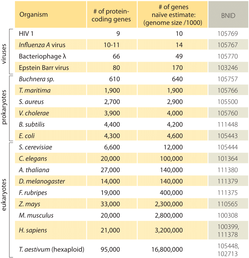
Table 1: A comparison between the number of genes in an organism and a naïve estimate based on the genome size divided by a constant factor of 1000bp/gene, i.e. predicted number of genes = genome size/1000. One finds that this crude rule of thumb works surprisingly well for many bacteria and archaea but fails miserably for multicellular organisms.
The simplest estimate of the number of genes in a genome unfolds by assuming that the entirety of the genome codes for genes of interest. To make further progress with the estimate, we need to have a measure of the number of amino acids in a typical protein which we will take to be roughly 300, cognizant however of the fact that like genomes, proteins come in a wide variety of sizes themselves as is revealed in the vignette on that topic, ”what are the sizes of proteins?”. On the basis of this meager assumption, we see that the number of bases needed to code for our typical protein is roughly 1000 (3 base pairs per amino acid). Hence, within this mindset, the number of genes contained in a genome is estimated to be the genome size/1000. For bacterial genomes, this strategy works surprisingly well as can be seen in table 1 and Figure 1. For example, when applied to the E. coli K-12, genome of 4.6 x 10⁶ bp, this rule of thumb leads to an estimate of 4600 genes, which can be compared to the current best knowledge of this quantity which is 4225. In going through a dozen representative bacteria and archeal genomes in the table a similarly striking predictive power to within about 10% is observed. On the other hand, this strategy fails spectacularly when we apply it to eukaryotic genomes, resulting for example in the estimate that the number of genes in the human genome should be 3,000,000, a gross overestimate. The unreliability of this estimate helps explain the existence of the Genesweep betting pool which as recently as the early 2000s had people betting on the number of genes in the human genome, with people’s estimates varying by more than a factor of ten.
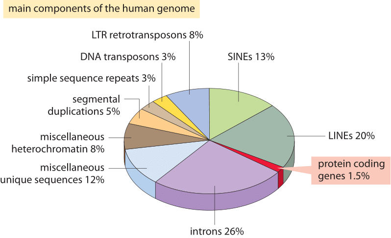
Figure 2: The different sequence components making up the human genome. About 1.5% of the genome consists of the ≈20,000 protein-coding sequences which are interspersed by the non coding introns, making up about 26%. Transposable elements are the largest fraction (40-50%) including for example long interspersed nuclear elements (LINEs), and short interspersed nuclear elements (SINEs). Most transposable elements are genomic remnants, which are currently defunct. (BNID 110283, Adapted from T. R. Gregory Nat Rev Genet. 9:699-708, 2005 based on International Human Genome Sequencing Consortium. Initial sequencing and analysis of the human genome. Nature 409:860 2001.)
What explains this spectacular failure of the most naïve estimate and what does it teach us about the information organized in genomes? Eukaryotic genomes, especially those associated with multicellular organisms, are characterized by a host of intriguing features that disrupt the simple coding picture exploited in the naïve estimate. These differences in genome usage are depicted pictorially in Figure 2 which shows the percentage of the genome used for other purposes than protein coding. As evident in Figure 1, prokaryotes can efficiently compact their protein coding sequences such that they are almost continuous and result in less than 10% of their genomes being assigned to non coding DNA (12% in E. coli, BNID 105750) whereas in humans over 98% (BNID 103748) is non protein coding.
The discovery of these other uses of the genome constitute some of the most important insights into DNA, and biology more generally, from the last 60 years. One of these alternative uses for genomic real estate is the regulatory genome, namely, the way in which large chunks of the genome are used as targets for the binding of regulatory proteins that give rise to the combinatorial control so typical of genomes in multicellular organisms. Another of the key features of eukaryotic genomes is the organization of their genes into introns and exons, with the expressed exons being much smaller than the intervening and spliced out introns. Beyond these features, there are endogenous retroviruses, fossil relics of former viral infections and strikingly, over 50% of the genome is taken up by the existence of repeating elements and transposons, various forms of which can perhaps be interpreted as selfish genes that have mechanisms to proliferate in a host genome. Some of these repeating elements and transposons are still active today whereas others have remained a relic after losing the ability to further proliferate in the genome.
In conclusion, genomes can be partitioned into two main classes: compact and expansive. The former are gene dense, with only about 10% of non-coding region and strict proportionality between genome size and genome number. This group extends to genomes of size up to about 10 Mbp, covering viruses, bacteria, archaea and some unicellular eukaryotes. The latter class shows no clear correlation between genome size and gene number, is composed mostly of non-coding elements and covers all multi-cellular organisms.