How many reactions do enzymes carry out each second?
One oversimplified and anthropomorphic view of a cell is as a big factory for transforming relatively simple incoming streams of molecules like sugars into complex biomass consisting of a mixture of proteins, lipids, nucleic acids and so on. The elementary processes in this factory are the metabolic transformations of compounds from one to another. The catalytic proteins taking part in these metabolic reactions, the enzymes, are almost invariably the largest fraction of the proteome of the cell (see www.proteomaps.net for a visual impression). They are thus also the largest component of the total cell dry mass. Using roughly one thousand such reactions, E. coli cells can grow on nothing but a carbon source such as glucose and some inorganic minerals to build the many molecular constituents of a functioning cell. What is the characteristic time scale (drum beat rhythm or clock rate, if you like) of these transformations?
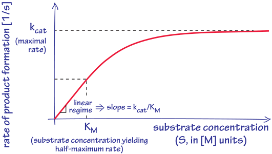
Figure 1: The characteristic dependence of enzyme catalysis rate on substrate concentration. Key defining effective parameters such as kcat, KM and their ratio, the second order rate constant that is equal to the slope at low concentrations, are denoted in the figure.
The biochemical reactions taking place in cells, though thermodynamically favorable, are in most cases very slow if left uncatalyzed. For example, the spontaneous cleavage of a peptide bond would take 400 years at room temperature and phosphomonoester hydrolysis, routinely breaking up ATP to release energy, would take about a million years in the absence of the enzymes that shuttle that reaction along (BNID 107209). Fortunately, metabolism is carried out by enzymes that often increase rates by an astonishing 10 orders of magnitude or more (BNID 105084, 107178). Phenomenologically, it is convenient to characterize enzymes kinetically by a catalytic rate kcat (also referred to as the turnover number). Simply put, kcat signifies how many reactions an enzyme can possibly make per unit time. This is shown schematically in Figure 1. Enzyme kinetics is often discussed within the canonical Michaelis-Menten framework but the so-called hyperbolic shape of the curves that characterize how the rate of product accumulation scales with substrate concentration feature several generic features that transcend the Michaelis-Menten framework itself. For example, at very low substrate concentrations, the rate of the reaction increases linearly with substrate concentration. In addition, at very high concentrations, the enzyme is cranking out as many product molecules as it can every second at a rate kcat and increasing the substrate concentration further will not lead to any further rate enhancement.
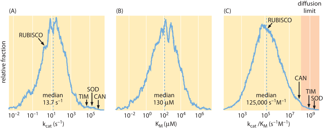
Figure 2. Distributions of enzyme kinetic parameters from the literature extracted from the BRENDA database: (A) kcat values (N = 1942), (B) kcat/KM values (N = 1882), and (C) KM values (N = 5194). Only values referring to natural substrates were included in the distributions. The location of several well-studied enzymes is highlighted: CAN, carbonic anhydrase; SOD, superoxide dismutase; TIM, triosephosphate isomerase; Rubisco, ribulose-1,5-bisphosphate carboxylase oxygenase. Adapted from Bar-Even et al, Biochemistry, 50(21):4402-4410, 2011.
Rates vary immensely. Record holders are carbonic anhydrase, the enzyme that transforms
CO2 into bicarbonate and back (CO2+H2OHCO3–+H+) and superoxide dismutase, an enzyme that protects cells against the reactivity of superoxide by transforming it into hydrogen peroxide (2O2–+2H+H2O2+O2). These enzymes can carry out as many as 106-107 reactions per second. At the opposite extreme, restriction enzymes limp along while performing only ≈10-1-10-2 reactions per second or about one reaction per minute per enzyme (BNID 101627, 101635). To flesh out the metabolic heartbeat of the cell we need a sense of the characteristic rates rather than the extremes. Figure 2A shows the distribution of kcat values for metabolic enzymes based on an extensive compilation of literature sources (BNID 111411). This figure reveals that the median kcat is about 10 s-1, several orders of magnitude lower than the common textbook examples, with the enzymes of central carbon metabolism, which is the cell’s metabolic highway, being on the average three times faster with a median of about 30 s-1.
How does one know if an enzyme works close to the maximal rate? From the general shape of the curve that relates enzyme rate to substrate concentration shown in Figure 1, there is a level of substrate concentration beyond which the enzyme will achieve more than half of its potential rate. The concentration at which the half-maximal rate is achieved is denoted KM. The definition of KM provides a natural measuring stick for telling us when concentrations are “low” and “high”. When the substrate concentration is well above KM, the reaction will proceed at close to the maximal rate kcat. At a substrate concentration [S]=KM the reaction will proceed at half of kcat. Enzyme kinetics in reality is usually much more elaborate than the textbook Michaelis-Menten model, with many enzymes exhibiting cooperativity and performing multi-substrate reactions of various mechanisms resulting in a plethora of functional forms for the rate law. But in most cases the general shape can be captured by the defining features of a maximal rate and substrate concentration at the point of half saturation as indicated schematically in Figure 1, meaning that the behavior of real enzymes can be cloaked in the language of Michaelis-Menten using kcat and KM, despite the fact that the underlying Michaelis-Menten model itself may not be appropriate.
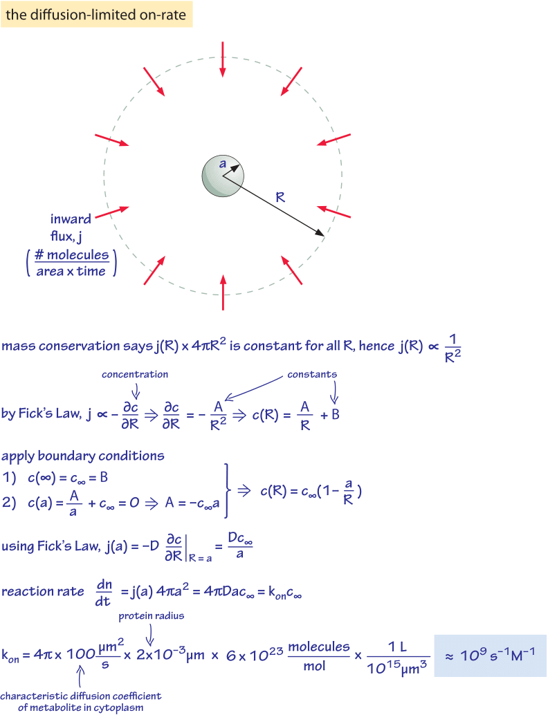
Figure 3: Derivation of the diffusion-limited on rate for example of metabolites to enzymes or of ligands to receptors.
We have seen that the actual rate depends upon how much substrate is present through the substrate affinity, KM. What are the characteristic values of KM for enzymes in the cell? As shown in Figure 2B, the median KM value is in the 0.1 mM range. From our rule of thumb (1nM is about 1 molecule per 1 E. coli volume) this is roughly equal to 100,000 substrate molecules per bacterial cell. At low substrate concentration ([S]<<KM) we can approximate the reaction rate by [ET]*kcat*[S]/KM, which is proportional to the product [ET]*[S] that measures the collision rate of the enzyme with the substrate with a proportionality rate factor of kcat/KM. This proportionality factor, known as the second order rate constant due to the fact that it multiplies two concentration terms, is the slope in Figure 1. This factor cannot be higher than the collision rate facilitated by diffusion unless electrostatic or other effects are in play. The value can be derived from the rules of diffusion as shown in Figure 3 and is known as the diffusion-limited rate. The idea of the calculation involves nothing more than working out the diffusive flux of substrate molecules onto our protein “absorber” and then asserting that every arriving molecule is able to undergo the reaction of interest. For a protein-sized enzyme and a small molecule substrate the diffusion-limited rate constant takes the value of roughly 109 s-1M-1. An enzyme approaching this limit can be described as optimal with respect to its ability to perform a successful transformation on every encounter provided by random diffusion. Few enzymes with notable exceptions such as the glycolytic enzyme triose isomerase (TIM) merit this status (BNID 103917). How well does the characteristic enzyme do? Figure 2C shows that the median value is about 105 s-1M-1, about 4 orders of magnitude lower than the diffusion limit. This difference can be partially explained by the liberal nature of the diffusion limit that does not depict all the issues related to binding and by noting that for many enzymes there might not be a strong selective pressure to optimize their kinetic properties. Moreover, the rate might be compromised in many cases by the need for recognition and specificity in the interaction.
The value of KM in conjunction with the diffusion-limited-on-rate can be used to estimate the off rates for bound substrate. The goal of the simple estimate is to find the time scale over which a substrate that is bound to the enzyme will stay bound before it goes back to solution (usually without reacting), the so called off rate koff. The estimate is based upon an ideal limit in which the on-rate is controlled by diffusive encounters with the enzyme characterized by the diffusion-limited-on-rate, kon ≈109 s-1M-1. An approximation for the koff is the product of this kon and the KM. So for example, if KM is a characteristic 10-4 M, the product is 105 s-1, so the substrate will unbind in about 10 μs, this is the so-called residence time. For extremely strong binders where the affinity is say 1 nM=10-9 M the residence time will be 1 s. This gives only a taste of the idealized case; the actual measured values for off-rates (or residence times) are revealed by enzymologists keeping them busy and confronted with a plethora of surprises. An analogous estimate for the off-rate can be considered for interactions between signaling molecules and for transcription factors binding to DNA with characteristic time scales from milliseconds to tens of seconds or even longer.
A striking quantitative insight into the possibilities and rate of interactions at the molecular level can be gleaned from a clever interpretation (D. S. Goodsell, “The machinery of life”, Springer, 2010) of the diffusion limit. Say we drop a test substrate molecule into a cytoplasm with a volume equal to that of a bacterial cell. If everything is well mixed and there is no binding, how long will it take for the substrate molecule to collide with one specific protein in the cell? The rate of enzyme substrate collisions is dictated by the diffusion limit which as shown above is equal to ≈109 s-1M-1 times the concentrations. We make use of one of our tricks of the trade which states that in E. coli a single molecule per cell (say our substrate) has an effective concentration of about 1nM (i.e. 10-9 M). The rate of collisions is thus 109 s-1M-1 x 10⁻⁹ M ≈ 1 s-1, i.e. they will meet within a second on average. This allows us to estimate that every substrate molecule collides with each and every protein in the cell on average about once per second. As a concrete example, think of a sugar molecule transported into the cell. Within a second it will have an opportunity to bump into all the different protein molecules in the cell. The high frequency of such molecular encounters is a mental picture worth carrying around when trying to have a grasp of the microscopic world of the cell.