How much cell-to-cell variability exists in protein expression?
It is tempting to discuss the absolute numbers or concentrations of expressed proteins within cells by assigning a single value, as opposed to speaking about distributions. Many methods for the measurement of protein quantity, for example measuring fluorescence using a spectrophotometer, supply only a single number that is an average over an entire population of cells. With the advent of quantitative microscopy and flow cytometry, both of which relied on the discovery of GFP, the role of variability has also moved to center stage. Functional roles for variability have already been shown in processes such as environmental responses where differences from one cell to the next effectively implement bet hedging, permitting some subset of a population to best adapt to some environmental insult. Yet the full implications and importance for the lifestyles of various organisms is still a hot area of research.
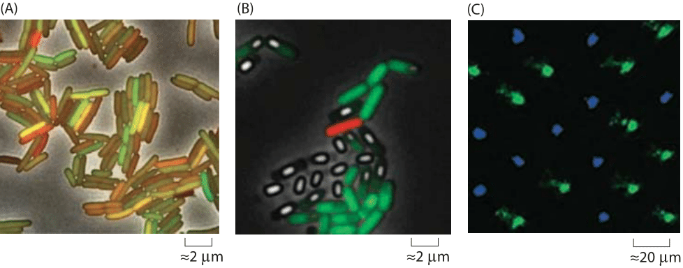
Figure 1: Examples of cell-to-cell variability in gene expression. (A) E. coli cells with identical promoters resulting in the production of fluorescent proteins with different colors. Noise results in a different relative proportion of red and green protein in each cell. (B) B. subtilis cells that are genetically identical adopt different fates despite the fact that they are subjected to identical conditions. The green cells are growing vegetatively, the white cells have sporulated and the red cells are in the “competent” state. (C) Drosophila retina revealing different pigments as revealed by staining photoreceptors with antibodies to different photopigments. The green-sensitive photopigment Rh6 is in green and the blue-sensitive photopigment Rh5 is in blue. (Adapted from (A) and (B) A. Eldar and M. B. Elowitz, Nature 467:267, 2010; (C) R. Losick and C. Desplan, Science, 320:65, 2008.)
If one performs an experiment in which single-cell microscopy is used to query the fluorescence in thousands of different cells as exemplified in Figure 1, a first stage in representing the data is by plotting the distribution. Figure 2 gives an example of such a distribution for the case of mRNAs. Many biological quantities display the log-normal distribution where the characteristic bell-shaped distribution is achieved when plotting the histogram in log scale. Different underlying mechanisms can result in such a distribution (A. L. Koch, JTB, 12:276, 1966). For example, a first-order kinetic parameter that is normally distributed and appears in the exponent of an autocatalytic growth processes will lead to a lognormal distribution. Alternatively, any characteristic that is the result of the multiplication of many other random processes is expected to be log-normally distributed due to the central limit theorem. A take home lesson is that one has to be very careful in making claims about the mechanism that gives rise to a given distribution. The reason is that often many different mechanisms can lead to the same generic distribution. Usually the next stage in characterization and data reduction is to calculate the statistics of a distribution, usually the mean and standard deviation. The level of variability in the population is usually given in terms of the coefficient of variation, the CV, equal to the ratio of the standard deviation to the mean. Alternatively, the Fano factor is the ratio of the variance (i.e the standard deviation squared) to the mean. This is of interest since it is known that for processes of a general form known as a Poisson process, the variance is predicted to be equal to the mean (Fano factor equal to 1), serving as a baseline expectation on the kind of noise that might be found for some promoters.
What is known about the actual levels of cell-cell variation in protein expression? Measurements based on fluorescent proteins have been the main tool for answering this question. Figure 1 shows how two-color experiments visually reveal the disparities in expression in bacteria. In this case, the lacI promoter was used to drive the expression of YFP and CFP genes integrated at opposing locations along the circular E. coli genome. In quantifying this variability one first has to note the approximately 2 fold change in size and content through the cell cycle. This is often corrected for by calculating a value normalized to the cell size. The amount of variability was quantified as having a characteristic CV for bacteria of ≈0.4 (BNID 107859) that could be further broken down into differences among cells and differences within a cell among identical promoters.
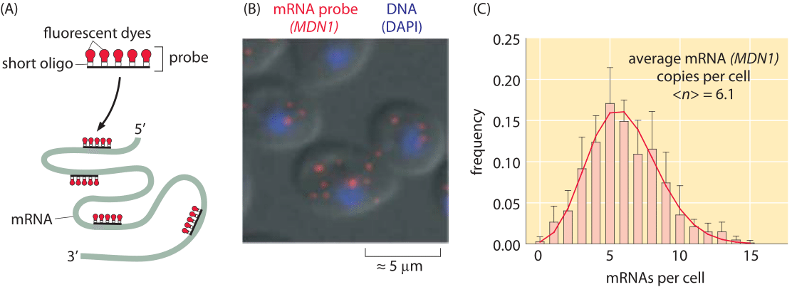
Figure 2: Measuring single cell variability of mRNA levels in budding yeast. (a) Cartoon showing how probes are designed to target different regions of an mRNA molecule of interest. (B) Fluorescence microscopy image of yeast cells revealing the number of mRNA per cell. (C) Histogram showing the number of mRNAs per cell for a particular gene (MDN1) of interest in yeast. (Adapted from D. Zenklusen et al., Nat Struct Mol Biol. 15:1263, 2008.)
What is known about the actual levels of cell-cell variation in protein expression? Measurements based on fluorescent proteins have been the main tool for answering this question. Figure 1 shows how two-color experiments visually reveal the disparities in expression in bacteria. In this case, the lacI promoter was used to drive the expression of YFP and CFP genes integrated at opposing locations along the circular E. coli genome. In quantifying this variability one first has to note the approximately 2 fold change in size and content through the cell cycle. This is often corrected for by calculating a value normalized to the cell size. The amount of variability was quantified as having a characteristic CV for bacteria of ≈0.4 (BNID 107859) that could be further broken down into differences among cells and differences within a cell among identical promoters.
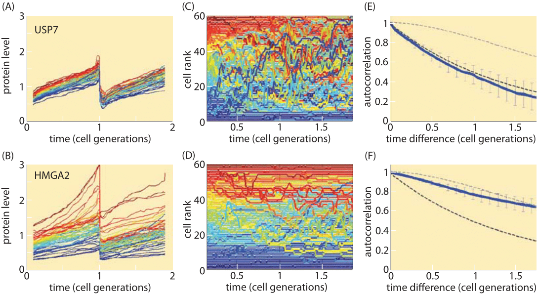
Figure 3: Variability and memory of protein levels in human cells. Different proteins have different levels of variability as well as differing rates of mixing within the population range. A, B. Time courses of fluorescent reporter levels indicating the levels of a protein over two cell cycles and showing the degree of variability among cells from the same cell line. The protein in the upper panel (USP7) is much less variable than the protein in the lower panel (HMGA2). C, D. Cells are ranked by level of expression of the tagged protein and their dynamics over time is made clear using a color code based on their level at the beginning of the first cell cycle. E, F. The rate of mixing of the protein levels within the cell population quantified by the autocorrelation function of protein levels as a function of time difference. Mixing times range from about one cell cycle to over two cell cycles. (Adapted from Sigal et al., Nature, 444:643, 2006.)
In human cells, similar measurements were undertaken with the CV values for a set of 20 proteins measured during the cell cycle. It was found that the CV was quite stable throughout the cell cycle while among proteins the values ranged from 0.1 to 0.3 (BNID 107860). As a rule of thumb, a log-normal distribution with a CV of ≈0.3 will have a ratio of ≈2 between the cells at the 90% percentile and the 10% percentile of expression intensity. One can go beyond the static “snapshot” level of variation to ask how quickly there is mixing within the population in which a cell that was a relatively low expresser becomes one of the high expressers as shown in Figure 3. Measuring such dynamics is based on time-lapse microscopy and the mixing time or memory timescale is quantified by the autocorrelation function that measures the average level of correlation between the levels at time t and t+τ, where τ denotes the time difference between the measurements. For protein levels in human cells, the memory time – the interval at which half of the correlation was lost, was between one and three generation times (BNID 108977, 107864), with some proteins mixing faster and others more slowly. Proteins with long mixing times can cause epigenetic behavior, where cells with identical genetic makeup respond differently, for example to chemotherapy treatment.