The Geography of the Cell
The vignettes which take center stage in the remainder of the book characterize many aspects of the lives of cells. There is no single path through the mass of data that we have assembled here, but nearly all of it refers to cells, their structures, the molecules that populate them and how they vary over time. As we navigate the numerical landscape of the cell, it is important to bear in mind that many of our vignettes are intimately connected. For example, when thinking about the rate of rotation of the flagellar motor that propels bacteria forward as discussed in the rates chapter, we will do well to remember that the energy source that drives this rotation is the transmembrane potential discussed in the energy and forces chapter. Further, the rotation of the motor is what governs the motility speed of those cells, a topic with quantitative enticements of its own. Though we will attempt to call out the reticular attachments between many of our different bionumbers, we ask the reader to be on constant alert for the ways in which our different vignettes can be linked up, many of which we probably did not notice and might harbor some new insights.
To set the cellular stage for the remainder of the book, in this brief section, we highlight three specific model cell types that will form the basis for the coming chapters. Our argument is that by developing intuition for the “typical” bacterium, the “typical” yeast cell and the “typical” mammalian cell, we will have a working guide for launching into more specialized cell types. For example, even when introducing the highly specialized photoreceptor cells which are the beautiful outcome of the evolution of “organs of extreme perfection” that so puzzled Darwin, we will still have our “standard” bacterium, yeast and mammalian cells in the back of our minds as a point of reference. This does not imply a naïveté on our side about the variability of these “typical” cells, indeed we have several vignettes on these very issues. It is rather an appreciation of the value of a quantitative mental description of a few standard cells that can serve as a useful benchmark to begin the quantitative tinkering that adapts to the biological case at hand, much as a globe gives us an impression of the relative proportion of our beloved planet that is covered by oceans and landmasses, and the key geographical features of those landmasses such as mountain ranges, deserts and rivers.
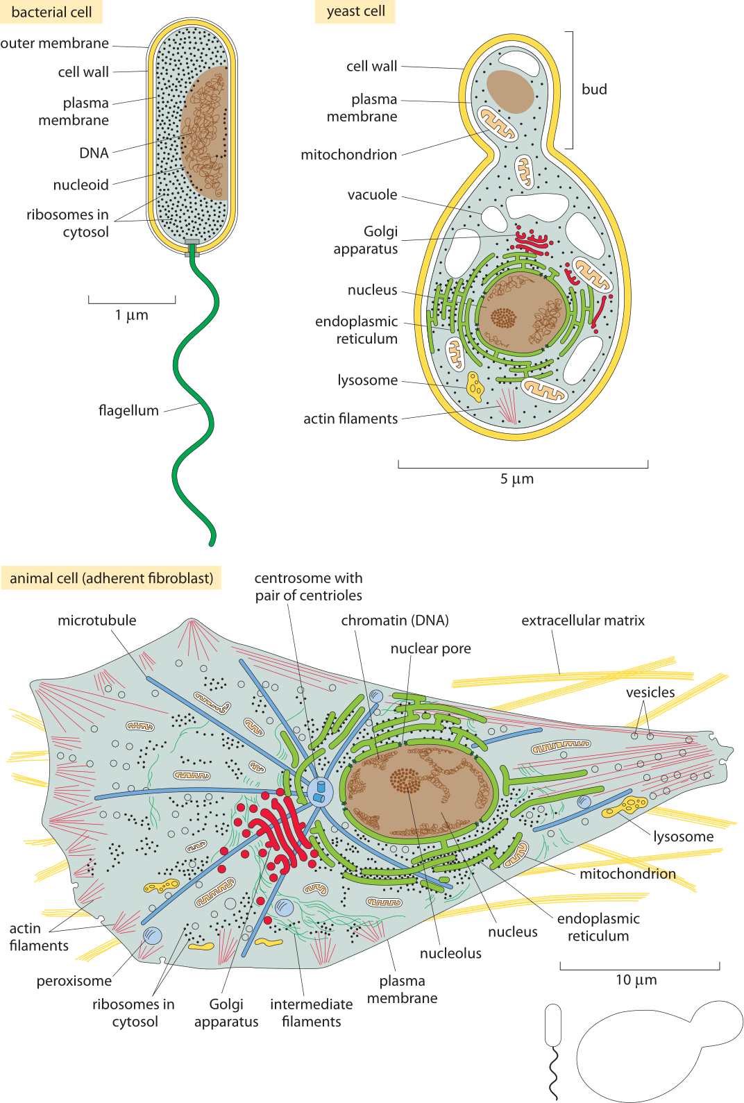
Figure 5: The Standard Cells. (A) A schematic bacterium revealing the characteristic size and components of E. coli. (B) A budding yeast cell showing its characteristic size, its organelles and various classes of molecules present within it. (C) An adherent human cell. We note that these are very simplified schematics so, for example, only a small fraction of ribosomes are drawn etc. Each cell is drawn to a different scale as indicated by the distinct scale bars in each schematic. The relative sizes of the bacterial and yeast cells at the same scale as the mammalian cell are shown in the bottom right. (Bacterium and animal cell adapted from Figs. 1.18 and 1.30 in B. Alberts et al., Molecular Biology of the Cell, 5th ed., New York, Garland Science, 2008)
Figure 4A shows us the structure of a bacterium such as the pet of nearly every molecular biologist, the famed E. coli. Figure 5A shows its molecular census. The yeast cell shown in Figures 5B and 6B reveals new layers of complexity beyond that seen in the standard bacterium as we see that these cells feature a variety of internal membrane-bound structures. One of the key reasons that yeast cells have served as representative of eukaryotic biology is the way they are divided into various compartments such as the nucleus, the endoplasmic reticulum and the Golgi apparatus. Further, their genomes are packed tightly within the cell nucleus in nucleoprotein complexes known as nucleosomes, an architectural motif shared by all eukaryotes. Beyond its representative cellular structures, yeast has been celebrated because of the “awesome power of yeast genetics”, meaning that in much the same way we can rewire the genomes of bacteria such as E. coli, we are now able to alter the yeast genome nearly at will. As seen in the table and figure, the key constituents of yeast cells can roughly be thought of as a scaled up version of the same census results already sketched for bacteria in Figure 5A.
Figure 5 gives a pictorial representation of our three standard cell types and Figure 6 complements it by showing the molecular census associated with each of those cell types. This figure goes hand in hand with Table 1 and can be thought of as a compact visual way of capturing the various numbers housed there. In some sense, much of the remainder of our book focuses on asking the questions: where do the numbers in these figures and that table come from? Do they make sense? What do they imply about the functional lives of cells? In what sense are cells the “same” and in what sense are they “different”?
Figures 5C and 6C complete the trifecta by showing a “standard” mammalian cell. The schematic shows the rich and heterogeneous structure of such cells. The nucleus houses the billions of base pairs of the genome and is the site of the critical transcription processes taking place as genes are turned on and off in response to environmental stimuli and over the course of both the cell cycle and development. Organelles such as the endoplasmic reticulum and the Golgi apparatus are the critical site of key processes such as protein processing and lipid biosynthesis. Mitochondria are the energy factories of cells where in humans, for example, about our body weight in ATP is synthesized each and every day. What can be said about the molecular players within these cells?
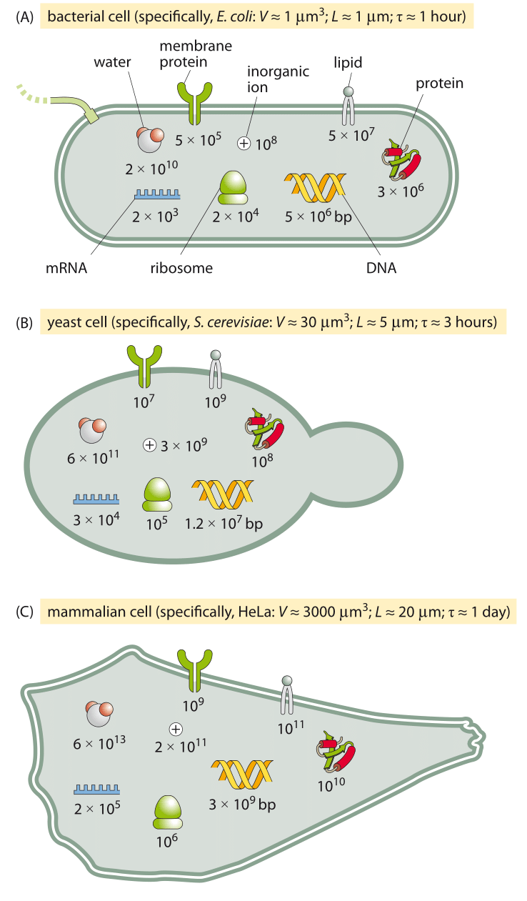
Figure 6: An order of magnitude census of the major components of the three model cells we employ often in the lab and in this book. A bacterial cell (E. coli), a unicellular eukaryote (the budding yeast S. cerevisiae, and a mammalian cell line (such as an adherent HeLa cell).
Let’s exemplify our thinking on a mammalian cell that has 1000 times the volume of a bacterial cell. Our first order expectation will be that the absolute copy number will be about 1000 times higher and the concentration stays about the same. The reader knows better than to take this as an immutable law. For example, some universal molecular players such as ribosomes or the total amount of mRNA also depend close to proportionally on the growth rate, i.e. inversely with the doubling time. For such a case we should account for the fact that the mammalian cell divides say 20 times slower than the bacterial cell. So for these cases we need a different null model. But in the alien world of molecular biology, where our intuition often fails any guidance (i.e. null model to rely on) can help. As a teaser example consider the question of how many copies there are of your favorite transcription factor in some mammalian cell line. Say P53 in a HeLa cell. From the rules of thumb above there are about 3 million proteins per µm3 and a characteristic mammalian cell will be 3,000 µm3 in volume. We have no reason to think our protein is especially high in terms of copy number, so it is probably not taking one part in a hundred of the proteome (only the most abundant proteins will do that). So an upper crude estimate would be 1 in a 1,000. This translates immediately into 3×10⁶ proteins/µm3 x 3000 µm3/ 1000 proteins/our protein ~ 10 million copies of our protein. As we shall see transcription factors are actually on the low end of the copy number range and something between 105-106 copies would have been a more accurate estimate, but we suggest this is definitely better than being absolutely clueless. Such an estimate is the crudest example of an easily acquired “sixth sense”. We find that those who master the simple rules of thumb discussed in this book have a significant edge in street-fighting cell biology (borrowing from Sanjoy Mahajan gem of a book on “street-fighting mathematics”).
Given that there are several million proteins in a typical bacterium and these are the product of several thousand genes, we can expect the “average” protein to have about 103 copies. The distribution is actually very far from being homogenous in any such manner as we will discuss in several vignettes in chapter 2 on concentrations and absolute numbers. Given the rule of thumb from above that one molecule per E. coli corresponds to a concentration of roughly 1 nM, we can predict the “average” protein concentration to be roughly 1 µM. We will be sure to critically dissect the concept of the “average” protein highlighting how most transcription factors are actually much less abundant than this hypothetical average protein and why components of the ribosome are needed in higher concentrations. We will also pay close attention to how to scale from bacteria to other cells. A crude and simplistic null model is to assume that the absolute numbers per cell tend to scale proportionally with the cell size. Under this null model, concentrations are independent of cell size.
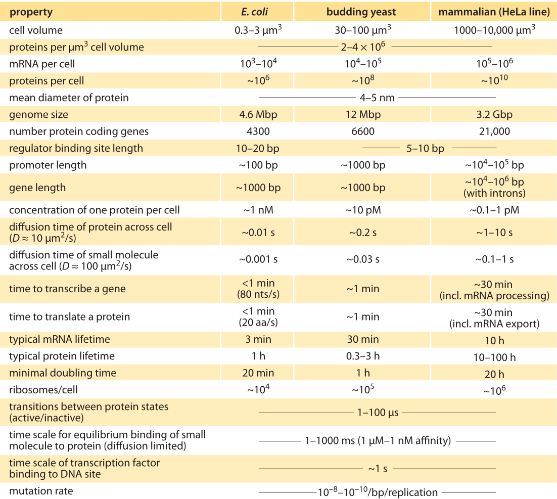
Table 1: Typical parameter values for a bacterial E. coli cell, the single-celled eukaryote S. cerevisiae (budding yeast), and a mammalian HeLa cell line. Note that these are crude characteristic values for happily dividing cells of the common lab strains. Adapted from U. Alon, “Introduction to Systems Biology”, CRC Press 2006. See full references at BNID 111494.
The logical development of the remainder of the book can be seen through the prism of Figure 5. First, we begin by noting the structures and their sizes. This is followed in the second chapter by a careful analysis of the copy numbers of many of the key molecular species found within cells. Already, at this point the interconnectedness of these numbers can be seen, for example, in the relation between the ribosome copy number and the cell size. In chapter 3, we then explore the energy and force scales that mediate the interactions between the structures and molecular species explored in the previous chapters. This is then followed in chapter 4 by an analysis of how the molecular and cellular drama plays out over time. Of course, the various structures depicted in Figure 5 exhibit order on many different scales, an order which conveys critical information to the survival and replication of cells. Chapter 5 provides a quantitative picture of different ways of viewing genomic information and on the fidelity of information transfer in a variety of different cellular processes. Our final chapter punctuates the diversity of cells way beyond what is shown in Figure 5 by characterizing the many cell types within a human body and considering a variety of other miscellany that defies being put into the simple conceptual boxes that characterize the other chapters.