What are the physical limits for detection by cells?

Living organisms have evolved a vast array of technologies for taking stock of conditions in their environment. Some of the most familiar and impressive examples come from our five senses. The “detectors” utilized by many organisms are especially notable for their sensitivity (ability to detect “weak” signals) and dynamic range (ability to detect both very weak and very strong signals). Hair cells in the ear can respond to sounds varying over more than 6 orders of magnitude in pressure difference between the detectability threshold (as low as 2 x 10^-10 atmospheres of sound pressure) and the onset of pain (6 x 10^-4 atmospheres of sound pressure). We note as an aside that given that atmospheric pressure is equivalent to pressure due to 10 meters of water, a detection threshold of 2 x 10^-10 atmospheres would result from the mass of a film of only 10 nm thickness, i.e. a few dozen atoms in height. Indeed, it is the enormous dynamic range of our hearing capacity that leads to the use of logarithmic scales (e.g. decibels) for describing sound intensity (which is the square of the change in pressure amplitude). The usage of a logarithmic scale is reminiscent of the Richter scale that permits us to describe the very broad range of energies associated with earthquakes. The usage of the logarithmic scale is also fitting as a result of the Weber-Fechner law that states that the subjective perception of many different kinds of senses, including hearing, is proportional to the logarithm of the stimulus intensity. Specifically, when a sound is a factor of 10ⁿ more intense than some other sound, we say that that sound is 10n decibels more intense. According to this law we perceive as equally different, sounds that differ by the same number of decibels. Some common sound levels, measured in decibel units, are shown in Figure 1. Given the range from 0 to roughly 130, this implies a dazzling 13 orders of magnitude. Besides this wide dynamic range in intensity, the human ear responds to sounds over a range of 3 orders of magnitude in frequency between roughly 20 Hz and 20,000 Hz, while at the same time being able to detect the difference between 440Hz and 441Hz.

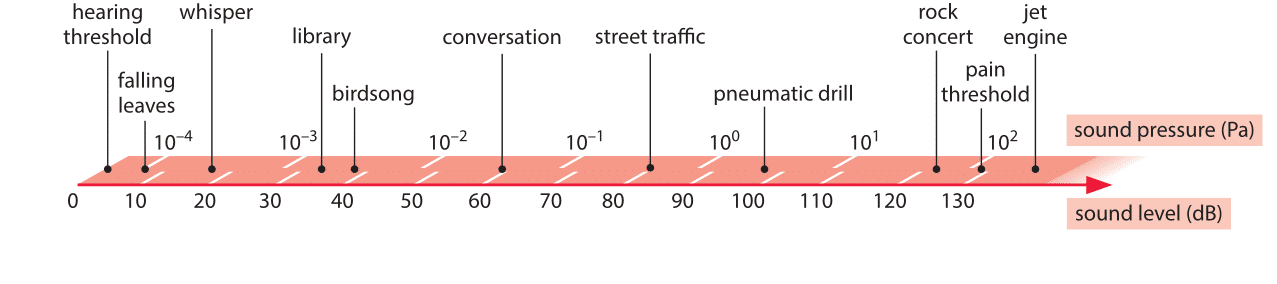
Figure 1: Intensities of common sounds in units of pressure and decibels.

Similarly impressively, rod photoreceptor cells can register the arrival of a single photon (BNID 100709, for cones a value of ≈100 is observed, BNID 100710). Here again the acute sensitivity is complemented by a dynamic range permitting us to see not only on bright sunny days but also on moonless starry nights with a 10⁹-fold lower illumination intensity.  A glance at the night sky in the Northern Hemisphere greets us with a view of the North Star (Polaris). In this case, the average distance between the photons arriving on our retina from that distant light source is roughly a kilometer, demonstrating the extremely feeble light intensity reaching our eyes (as well as how fast the speed of light is….).

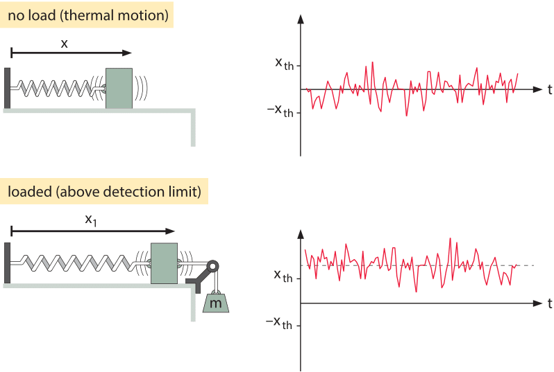
Figure 2: Deflection of a mass-spring system. In the top panel, there is no applied force and the mass moves spontaneously on the frictionless table due to thermal fluctuations. In the lower panel, a force is applied to the mass-spring system by hanging a weight on it. The graphs show the position of the mass as a function of time revealing both the stochastic and deterministic origins of the motion. As shown in the lower panel, in order to have a detectable signal, the mean displacement needs to be above the amplitude of the thermal motions.

Through studying the observed minimum stimuli detected by cells, we can ask if evolution drove organisms all the way to the limit dictated by physics. To begin to see how the challenge of constructing sensors with high sensitivity and wide dynamic range plays out, we consider the effects of temperature on an idealized tiny frictionless mass-spring system as shown in Figure 2 where the spring is characterized by a spring constant k. The goal is to measure the force applied on the mass. It is critical to understand how noise influences our ability to make this measurement. The mass will be subjected to constant thermal jiggling as a result of collisions with the molecules of the surrounding environment as well as other internal processes within the spring itself. As an extension to the discussion in the vignette on “What is the thermal energy scale and how is it relevant to biology?”, the energy resulting from these collisions equals ½ k_BT, where k_B is Boltzmann’s constant and T is the temperature in degrees Kelvin. What this means is that the mass will spontaneously jiggle around its equilibrium position as shown in Figure 2, with the deflection x set by the condition that

As noted above, just like an old-fashioned scale used to measure the weight of fruits or humans, the way we measure the force is by reading out the displacement of the mass. Hence, in order for us to measure the force, the displacement must exceed a threshold set by the thermal jiggling.  That is, we can only say that we have measured the force of interest once the displacement exceeds the displacements that arise spontaneously from thermal fluctuations or

Imposing this constraint results in x_min=(k_BT/k)^1/2, which gives a force limit F_min=(kk_BT)^1/2. This limit states that we cannot measure smaller forces because the displacements they engender could just as well have come from thermal agitation. One way to overcome these limits is to increase the measurement time (which depends on the spring constant). Many of the most clever tools of modern biophysics such as the optical trap and atomic-force microscope are designed both to overcome and exploit these effects.

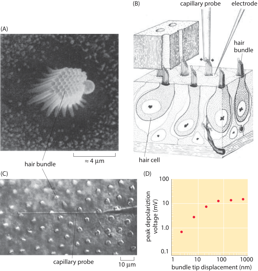
Figure 3: Response of hair cells to mechanical stimulation. (A) Bundle of stereocillia in the cochlea of a bullfrog. (B) Schematic of the experiment showing how the hair bundle is manipulated mechanically by the capillary probe and how the electrical response is measured using an electrode. (C) Microscopy image of cochlear hair cells from a turtle and the capillary probe used to perturb them. (D) Voltage as a function of the bundle displacement for the hair cells shown in part (C). (Adapted from (A) A. J. Hudspeth, Nature, 341:398, 1989. (B) A. J. Hudspeth and D. P. Corey,, Proc. Nat. Acad. Sci., 74:2407, 1977. (C) and (D) A. C. Crawford and R. Fettiplace , J. Physiol. 364:359, 1985.)

To give a concrete example, we consider the case of the hair cells of the ear. Each such hair cell features a bundle of roughly 30-300 stereocilia as shown in Figure 3. These stereocilia are approximately 10 microns in length (BNID 109301, 109302). These small cellular appendages serve as springs that are responsible for transducing the mechanical stimulus from sound and converting it into electrical signals that can be interpreted by the brain. In response to changes in air pressure, the stereocilia are subjected to displacements that result in the gating of ion channels which leads in turn to further signal transduction. Different stereocilia respond at different frequencies which makes it possible for us to distinguish the melodies of Beethoven’s Fifth Symphony from the cacophony of a car horn. The mechanical properties of the stereocilia are similar to those of the spring that was discussed in the context of Figure 2. By pushing on individual stereocilium with a small glass fiber as shown in Figure 3, it is possible to measure the minimal displacements of the stereocilia that can trigger a detectable change in voltage. Rotation of the hair bundle by only 0.01 degree, corresponding to nanometer-scale displacements at the tip, are sufficient to elicit a voltage response of mV scale (BNID 111036, 111038).  How do these numbers compare to those expected from thermal jiggling of the stereocilia? Both the observed Brownian motion as well as simple theoretical estimates using spring models like that described above reveal thermal motions of the stereocilia tips that are several nanometers in size. However, the hearing threshold appears to correspond to displacements of as little as 0.1 nm as seen in Figure 3. This interesting discrepancy actually points to the fact that the hair bundle is active and amplifies input close to its resonance frequency as well as the fact that the stereocilia are coupled, effects not considered in the simple estimate.

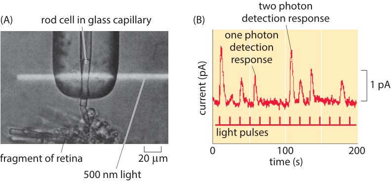
Figure 4: Single-photon response of individual photoreceptors. (A) Experimental setup shows a single rod cell from the retina of a toad in a glass capillary and subjected to a beam of light. (B) Current traces as a function of time for photoreceptor subjected to light pulses in an experiment like that shown in part (A). (Adapted from (A) D. A. Baylor, et al., J. Physiol., 288:589, 1979; (B) F. Rieke and D. A. Baylor, Rev. Mod. Phys., 70:1027, 1998. )

This same kind of reasoning governs the physical limits for our other senses as well. Namely, there is some intrinsic noise added to the property of the system we are measuring. Hence, to get a “readout” of some input, the resulting output has to be larger than the natural fluctuations of the output variable. For example, the detection and exploitation of energy carried by photons is linked to some of life’s most important processes including photosynthesis and vision.  How many photons suffice to result in a change in the physiological state of a cell or organism? In now classic experiments on vision, the electrical currents from individual photoreceptor cells stimulated by light were measured. Figure 4 shows how a beam of light was applied to individual photoreceptors and how electric current traces from such experiments were measured. The experiments revealed two key insights. First, photoreceptors undergo spontaneous firing, even in the absence of light, revealing precisely the kind of noise that real events (i.e. the arrival of a photon) have to compete against. In particular, these currents are thought to result from the spontaneous thermal isomerization of individual rhodopsin molecules as discussed in the vignette on “How many rhodopsin molecules are in a rod cell?”. This isomerization reaction is normally induced by the arrival of a photon and results in the signaling cascade we perceive as vision. Second, examining the quantized nature of the currents emerging from photoreceptors exposed to very weak light demonstrates that such photoreceptors can respond to the arrival of a single photon. This effect is shown explicitly in Figure 4B.

Another class of parameters that are “measured” with great sensitivity by cells includes the absolute numbers, identities and gradients of different chemical species. This is a key requirement in the process of development where a gradient of morphogen is translated into a recipe for pattern formation. A similar interpretation of molecular gradients is important for motile cells as they navigate the complicated chemical landscape of their watery environment. These impressive feats are not restricted to large and thinking multicellular organisms such as humans. Even individual bacteria can be said to have “knowledge” of their environment as illustrated in the exemplary system of chemotaxis already introduced in the vignette on “What are the absolute numbers of signaling proteins”. That “knowledge” leads to purposeful discriminatory power where even a few molecules of attractant per cell can be detected and amplified and differences in concentrations over a wide dynamic range of about 5 orders of magnitude can be amplified (BNID 109306, 109305). This enables unicellular behaviors in which individual bacteria will swim up a concentration gradient of chemoattractant. To get a sense of the exquisite sensitivity of these systems, Figure 5 gives a simple calculation of the concentrations being measured by a bacterium during the chemotaxis process and estimates the changes in occupancy of a surface receptor that is detecting the gradients. In particular, if we think of chemical detection by membrane-bound protein receptors, the way that the presence of a ligand is read out is by virtue of some change in the occupancy of that receptor. As the figure shows, a small change in concentration of ligand leads to a corresponding change in the occupancy of the receptor. For the case of bacterial chemotaxis, a typical gradient detected by bacteria in a microscopy experiment can be reasoned out as follows. If we consider bacteria swimming roughly 1 mm away from a pipette with 1 mM concentration of chemoattractant, the gradient is of order 10-2 M/m (BNID 111492). Is such a gradient big or small? A single-molecule difference detection threshold can be defined as:

Interestingly, recent work has demonstrated that bacteria can even detect gradients smaller than this (though an attendant insight is that the quantity actually being “measured” by the cells is actually the gradient of the logarithm of the concentration). As noted above, this small gradient can be measured over a very wide range of absolute concentrations, illustrating both the sensitivity and dynamic range of this process, but also revealing a more nuanced mechanism than the simple occupancy hypothesis described in Figure 5 since like with the hair cell example discussed earlier in the vignette, chemotaxis receptors are adaptive. These same type of arguments arise in the context of development where morphogen gradient interpretation is based upon nucleus-to-nucleus measurement of concentration differences. For example, in the establishment of the anterior-posterior patterning of the fly embryo, neighboring nuclei are “measuring” roughly 500 and 550 molecules per nuclear volume and using that difference to make decisions about developmental fate.

In summary, evolution pushed cells to detect environmental signals with both exquisite sensitivity and impressive dynamic range. In this process physical limits must be respected but cells find creative solutions. Photoreceptors can detect individual photons, the olfactory system nears the single-molecule detection limit, hair cells can detect pressure differences as small as 10^-9 atm and bacteria can detect gradients that correspond to less than one molecule per cell per cell length, a dazzling display of subtle and beautiful mechanisms.

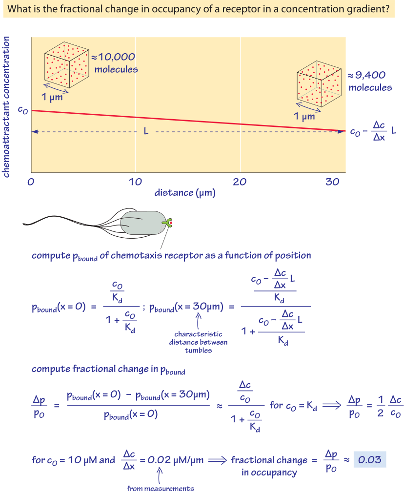
Figure 5: Back of the envelope calculation