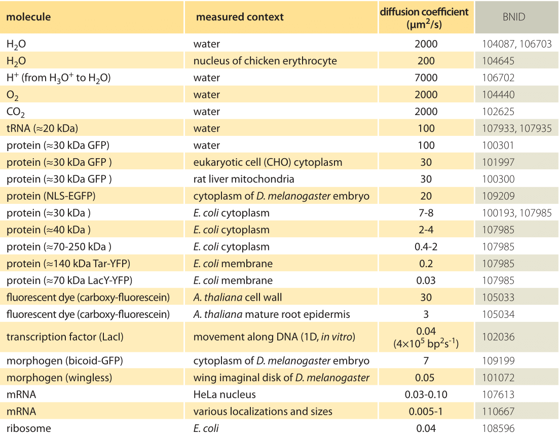
Table 1: A compilation of empirical diffusion constants showing the dependence on size and cellular context

One of the most pervasive processes that serves as the reference time scale for all other processes in cells is that of diffusion. Molecules are engaged in an incessant, chaotic dance, as characterized in detail by the botanist Robert Brown in his paper with the impressive title “A Brief Account of Microscopical Observations Made in the Months of June, July, and August, 1827, On the Particles Contained in the Pollen of Plants, and on the General Existence of Active Molecules in Organic and Inorganic Bodies”.  The subject of this work has been canonized as Brownian motion in honor of Brown’s seminal and careful measurements of the movements bearing his name. As he observed, diffusion refers to the random motions undergone by small scale objects as a result of their collisions with the molecules making up the surrounding medium.

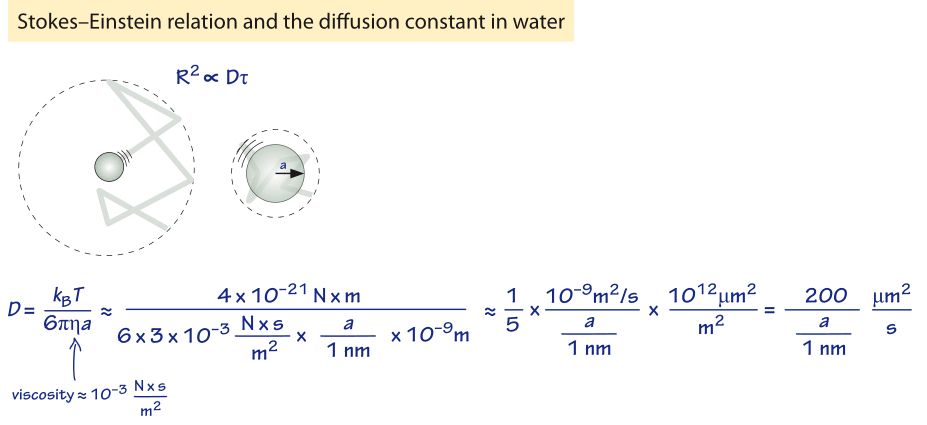
Figure 1: Back of the envelope estimate for the diffusion constant of a sphere of radius a in water.

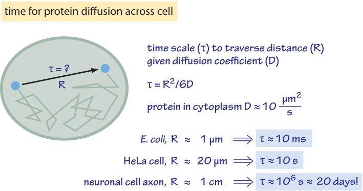
Figure 2: Back of the envelope estimate for the time scale to traverse a cell by diffusion. We assume a characteristic diffusion coefficient for a monomeric protein of 30 kDa. At higher molecular mass there is a reduction of about an order of magnitude as shown in Table 1 and the time scales will increase by the same factor. The protein diffusion constant used to estimate time scales within cells takes into account an order of magnitude reduction in the diffusion constant in the cell relative to its value in water. The factor of 6 in the denominator of the equation for τ applies to diffusion in three dimensions. In the two- or one-dimensional cases, it should be replaced with 4 or 2, respectively. The mammalian cell characteristic distance is taken to be 20 μm, characteristic of spreading adherent cells.

The study of diffusion is one of the great meeting places for nearly all disciplines of modern science. In both chemistry and biology, diffusion is often the dynamical basis for a broad spectrum of different reactions. The mathematical description of such processes has been one of the centerpieces of mathematical physics for nearly two centuries and permits the construction of simple rules of thumb for evaluating the characteristic time scales of diffusive processes. In particular, the concentration of some diffusing species as a function of both position and time is captured mathematically using the so-called diffusion equation. The key parameter in this equation is the diffusion constant, D, with larger diffusion constants indicating a higher rate of jiggling around. The value of D is microscopically governed by the velocity of the molecule and the mean time between collisions. One of the key results that emerges from the mathematical analysis of diffusion problems is that the time scale τ for a particle to travel a distance x is given on the average by τ ≈ x²/D, indicating that the dimensions of the diffusion constant are length²/time. This rule of thumb shows that the diffusion time increases quadratically with the distance, with major implications for processes in cell biology as we now discuss.

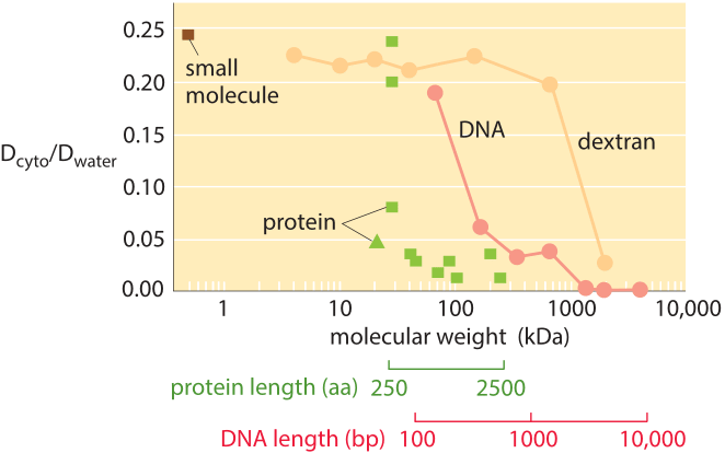
Figure 3: The decrease in the diffusion constant in the cytoplasm with respect to water as molecular weight increases. For the different proteins marked in green see Kumar et al 2010 and entries in the compilation table below. (Adapted from A. S. Verkman, Trends Biochem., 27:27, 2002; M. Kumar et al., Biophysical Journal, 98:552, 2010).

How long does it take macromolecules to traverse a given cell? We will perform a crude estimate. As derived in Figure 1, the characteristic diffusion constant for a molecule the size of a monomeric protein is ≈100 µm²/s in water and is about ten-fold smaller, ≈10 µm²/s, inside a cell with large variations depending on the cellular context as shown in Table 1 (larger proteins often show another order of magnitude decrease to ≈1 µm²/s, BNID 107985). Using the simple rule of thumb introduced above, we find as shown in Figure 2 that it takes roughly 0.01 seconds for a protein to traverse the 1 micron diameter of an E. coli cell (BNID 103801). A similar calculation results in a value of about 10 seconds for a protein to traverse a HeLa cell (adhering HeLa cell diameter ≈20 µm, BNID 103788).  An axon 1 cm long is about 500 times longer still and from the diffusion time scaling as the square of the distance it would take 10⁶ seconds or about two weeks for a molecule to travel this distance solely by diffusion. This enormous increase in diffusive time scales as cells approach macroscopic sizes demonstrates the necessity of mechanisms other than diffusion for molecules to travel these long distances. Using a molecular motor moving at a rate of ≈1 µm/s (BNID 105241) it will take a “physiologically reasonable” 2-3 hours to traverse this same distance. For extremely long neurons, that can reach a meter in length in a human (or 5 meters in a giraffe), recent research raises the speculation that neighboring glia cells alleviate much of the diffusional time limits by exporting cell material to the neuron periphery from their nearby position (K. A. Nave, Nat. Rev. Neuroscience, 11:275, 2010). This can decrease the time for transport by orders of magnitude but also requires dealing with transport across the cell membrane.

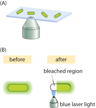
Figure 4: Fluorescence recovery after photobleaching in bacteria. (A) Schematic of how the FRAP technique works. The laser photobleaches the fluorescent proteins in a selected region. Because of diffusion, proteins that were not bleached come into the bleached region over time. (B) Higher resolution schematic of the photobleaching process over a selected region within the cell.

How much slower is diffusion in the cytoplasm in comparison to water and what are the underlying causes for this difference? Measurements show that the cellular context affects diffusion rates by a factor that depends strongly on the compound’s biophysical properties as well as size. For example, small metabolites might suffer only a 4-fold decrease in their diffusive rates, whereas DNA can exhibit a diffusive slowing down in the cell that is tens or hundreds of times slower than in water as shown in Figure 3. Causes for these effects have been grouped into categories and explained by analogy to an automobile (A. S. Verkman, Trends Biochem. Sci., 27:27,  2002): the viscosity (like drag due to car speed), binding to intracellular compartments (time spent at stop lights) and collisions with other molecules also known as molecular crowding (route meandering). Recent analysis (T. Ando & J. Skolnick, Proc. Natl. Acad. Sci., 107:18457, 2010) highlights the importance of hydrodynamic interactions – the effects of moving objects in a fluid on other objects similar to the effect of boats on each other via their wake. Such interactions lead approaching bodies to repel each other whereas two bodies that are moving away are attracted.

Complications like those described above make the study of diffusion in living cells very challenging.  To the extent that these processes can be captured with a single parameter, namely, the diffusion coefficient, one might wonder how are these parameters actually measured? One interesting method turns one of the most annoying features of fluorescent proteins into a strength. When exposed to light, fluorescent molecules lose their ability to fluoresce over time. But this becomes a convenience when the bleached region is only part of a cell. The reason is that after the bleaching event, because of the diffusion of the unbleached molecules from other regions of the cell, they will fill in the bleached region, thus increasing  the fluorescence (the so called “recovery” phase in in FRAP). This idea is shown schematically in Figure 4. Using this technique, systematic studies of the dependence of the diffusion coefficient on molecular size for cytoplasmic proteins in E. coli have been undertaken, with results as shown in Figure 5, illustrating the power of this method to discriminate the diffusion of different proteins in the bacterial cytoplasm.

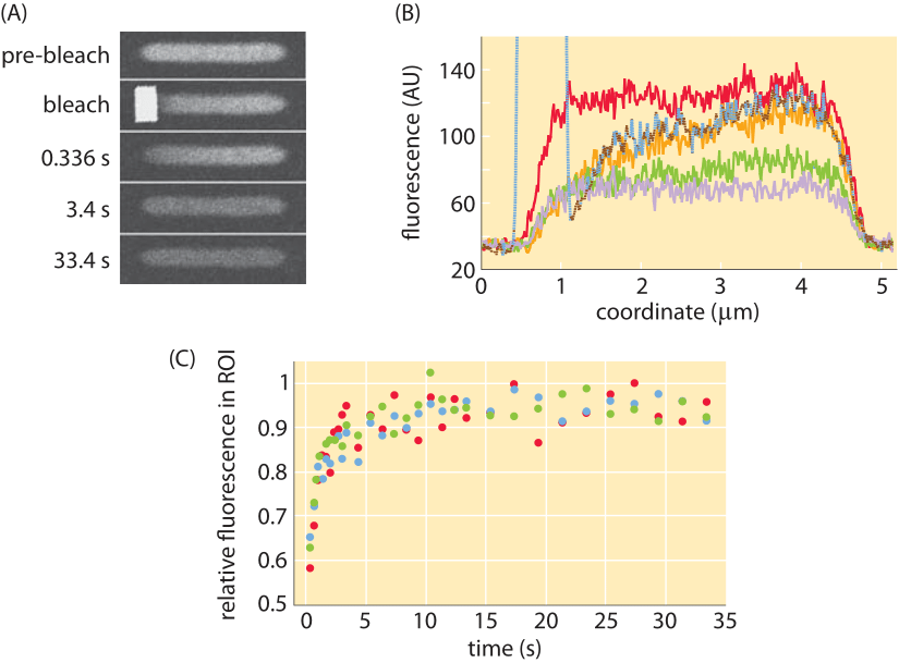
Figure 5: Fluorescence recovery after photobleaching in E. coli cells. (A) Images of E. coli cells before and after the bleaching process showing the spatial distribution of fluorescence. (B) Fluorescence as a function of position for different times. (C) Recovery of fluorescence over time as measured in multiple experiments. (Adapted M. Kumar et al., Biophysical Journal, 98:552, 2010)

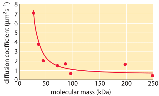
Figure 6: Diffusion constant as a function of molecular mass in E. coli. The diffusion of proteins within the E. coli cytoplasm were measured using the FRAP technique. (Adapted M. Kumar et al., Biophysical Journal, 98:552, 2010)